CS 180: Final Project
Tour Into the Picture and Light Field Camera
Meenakshi Mittal
The first project we will take a look at is tour into the picture, where we create 3-dimensional models of 2-dimensional images with one point perspective. The second project is light field camera, where we use grids of images from the Stanford Light Field Archive to focus an image at different depths and adjust aperture.
Project 1: Tour Into the Picture
This project requires that we use images with one point perspective. I selected the following 4 images to model in 3D, 2 of which are paintings and 2 of which I captured myself:
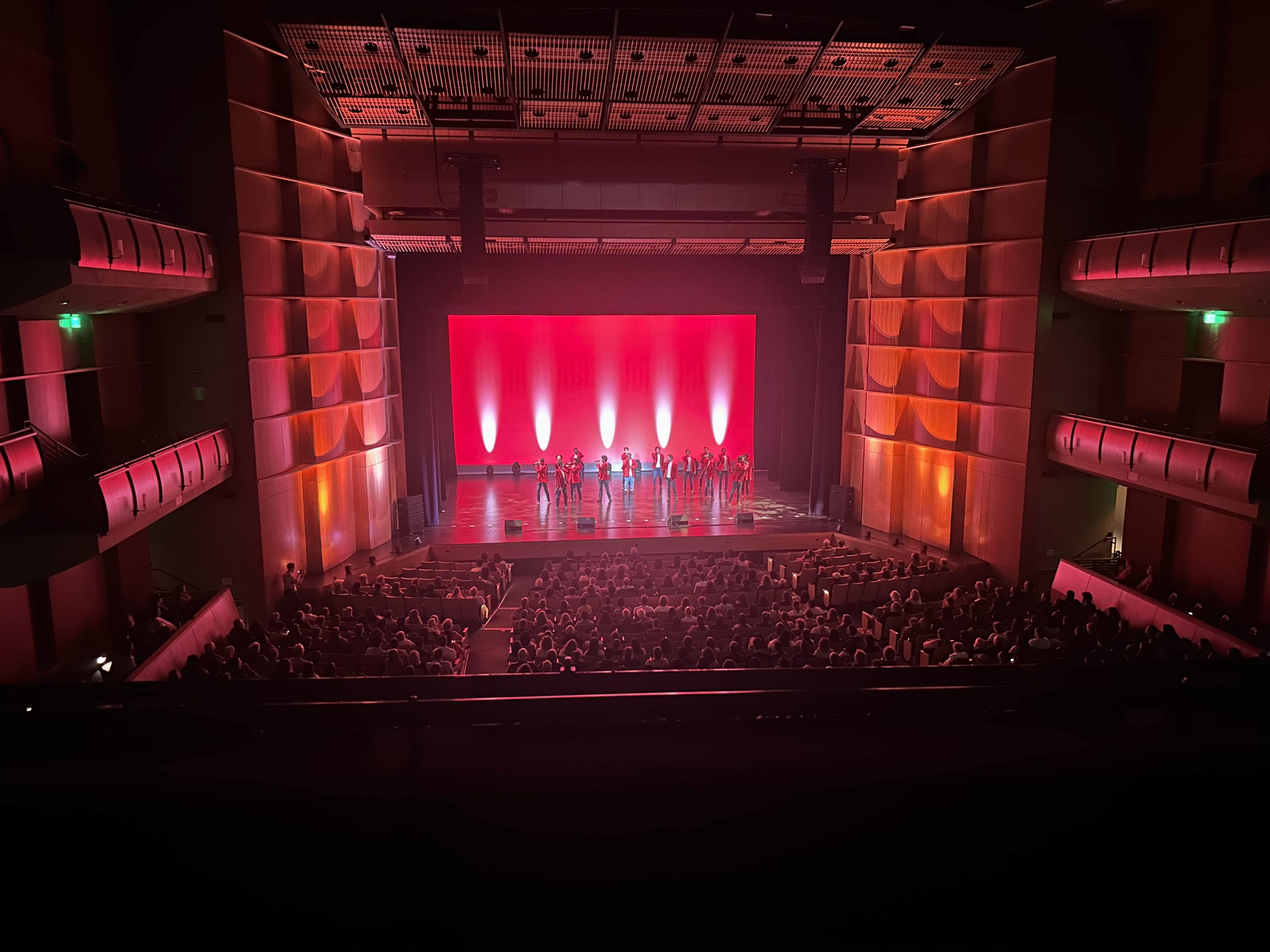
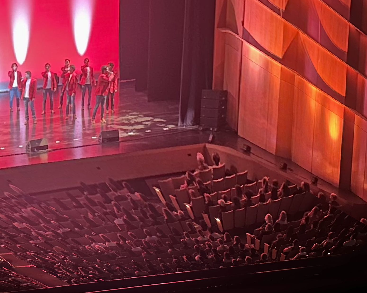
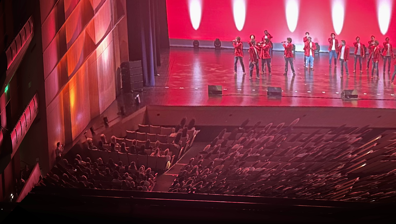
Acapella Show
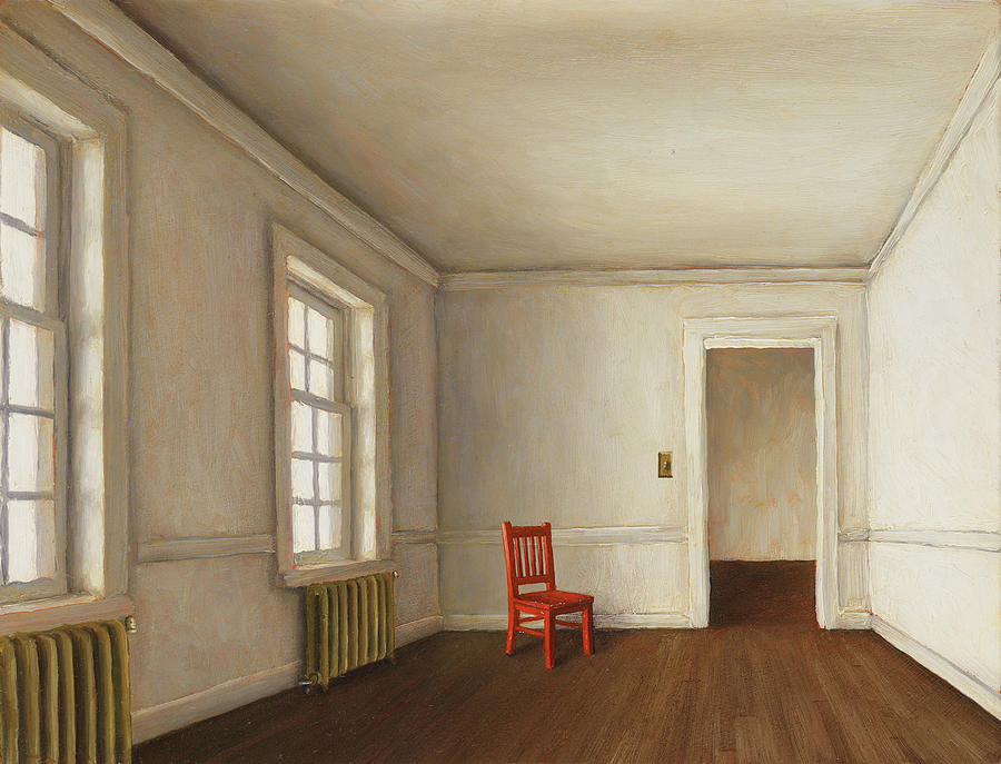
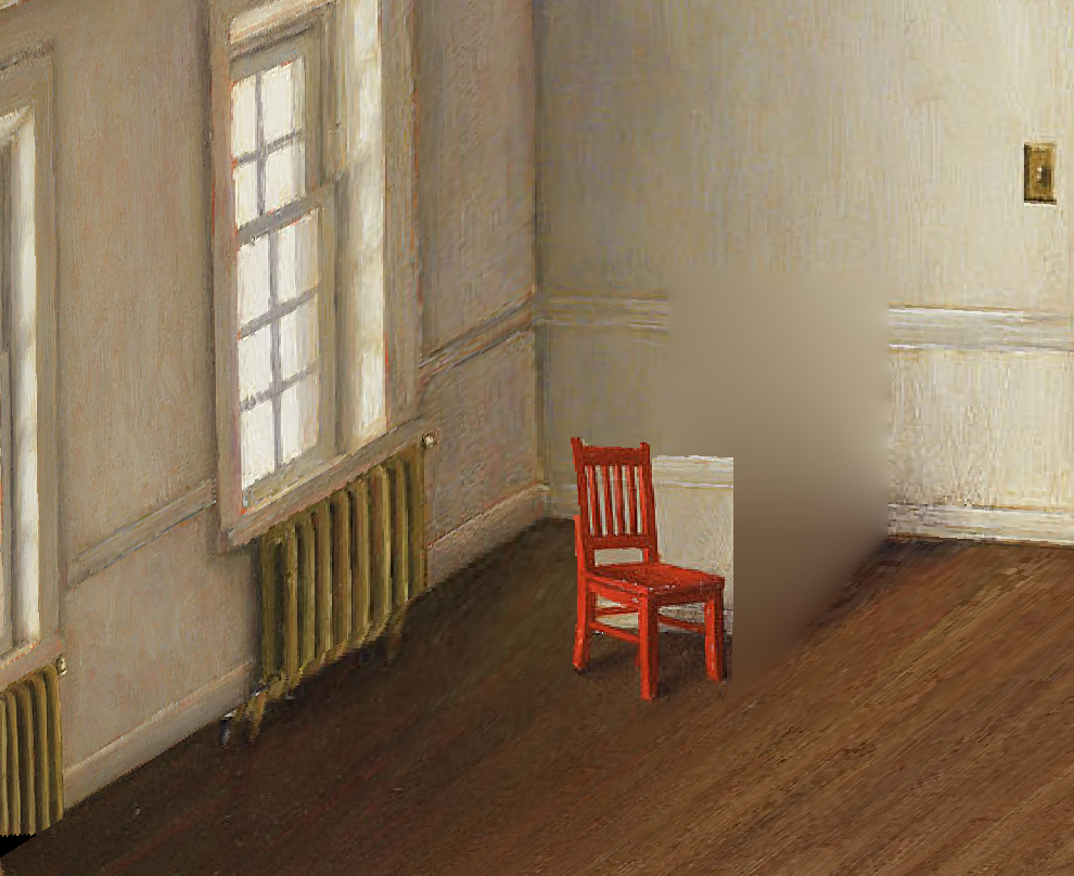
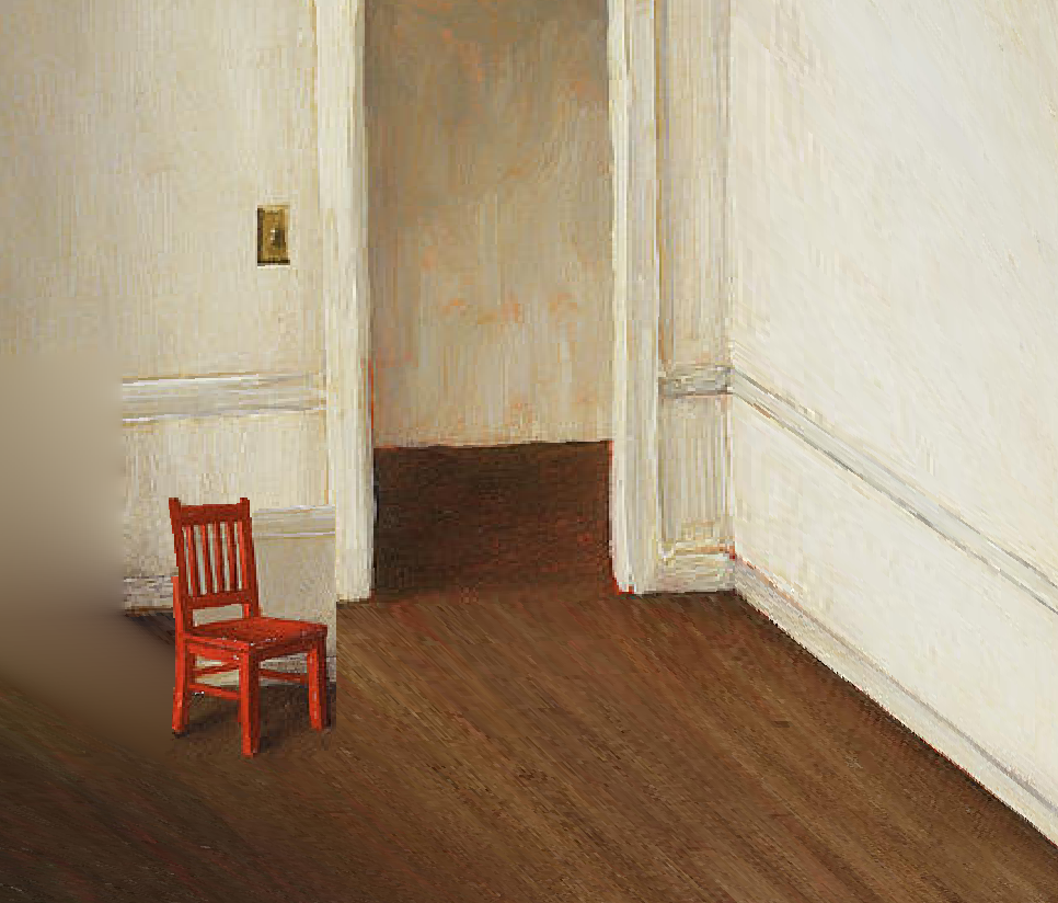
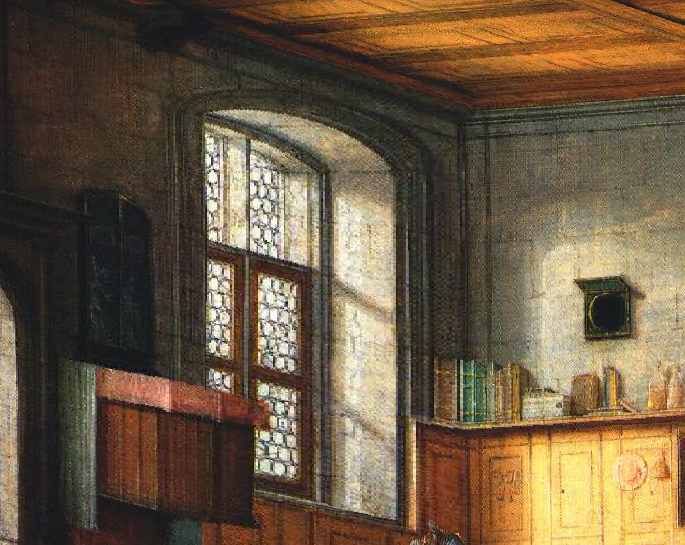
White Room - Harry Steen
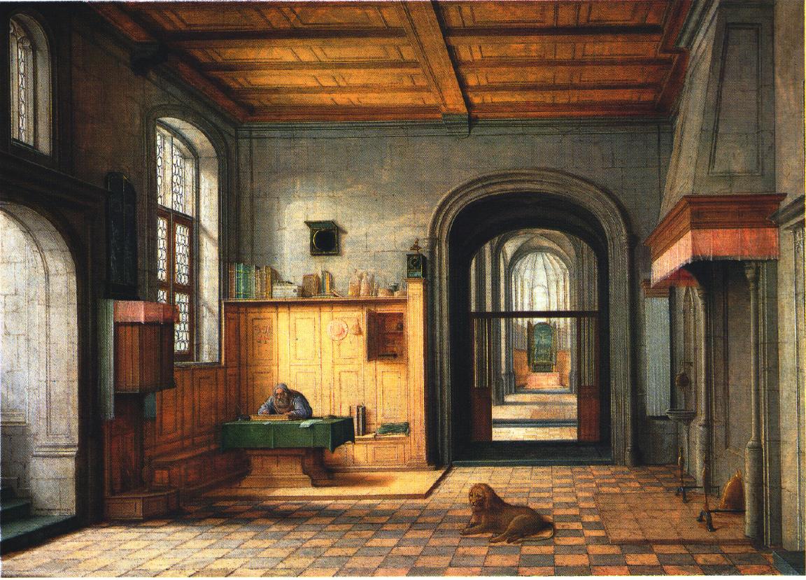
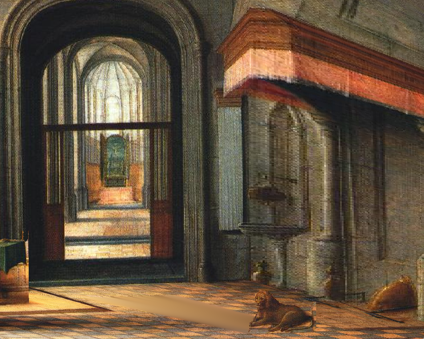
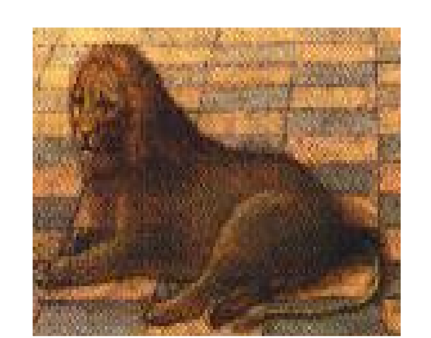
St. Jerome - Henry Steinwick
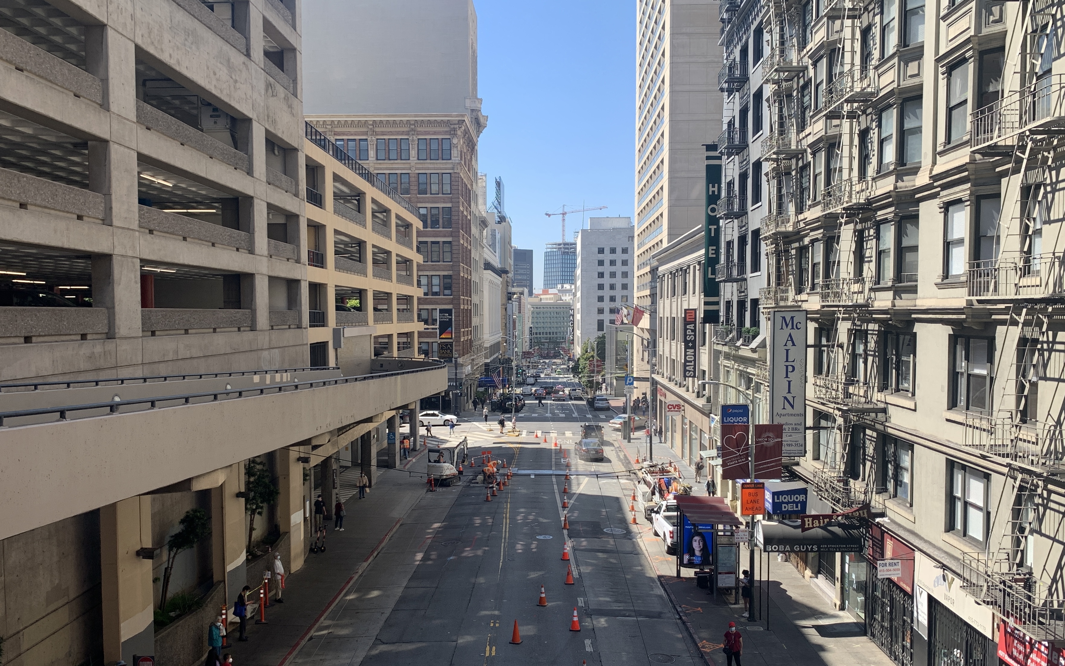
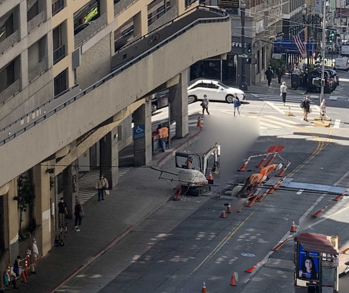
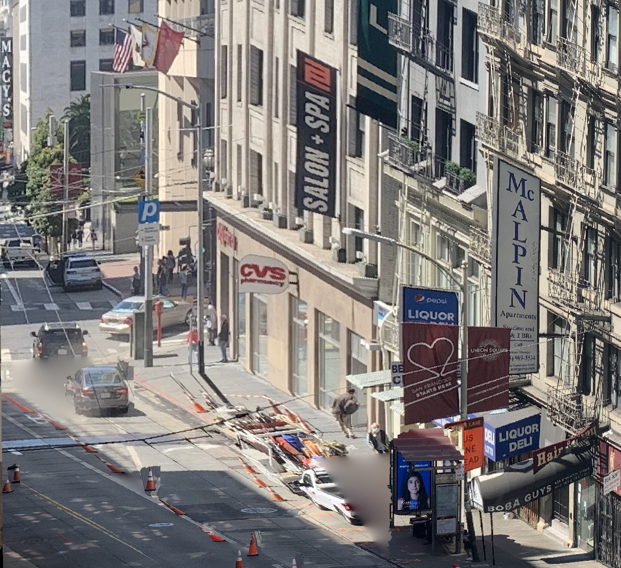
San Francisco
The first step is to identify the 5 planes of the images that we wish to reconstruct. These planes are the back wall, left wall, right wall, floor, and ceiling. The provided MATLAB starter code helps us identify these walls by specifying the back wall and vanishing point. The plane segmentation is shown here (the lines are thin-- I suggest zooming in to see them):
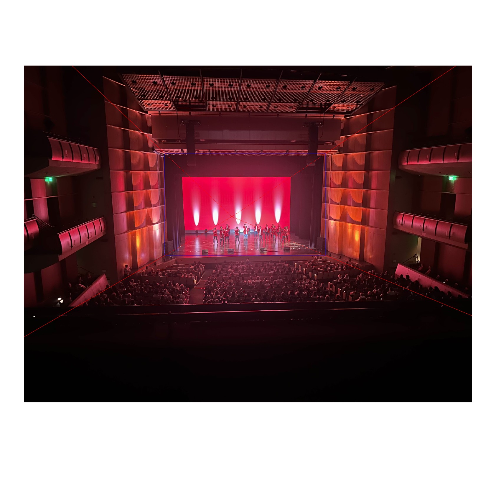
Acapella Show
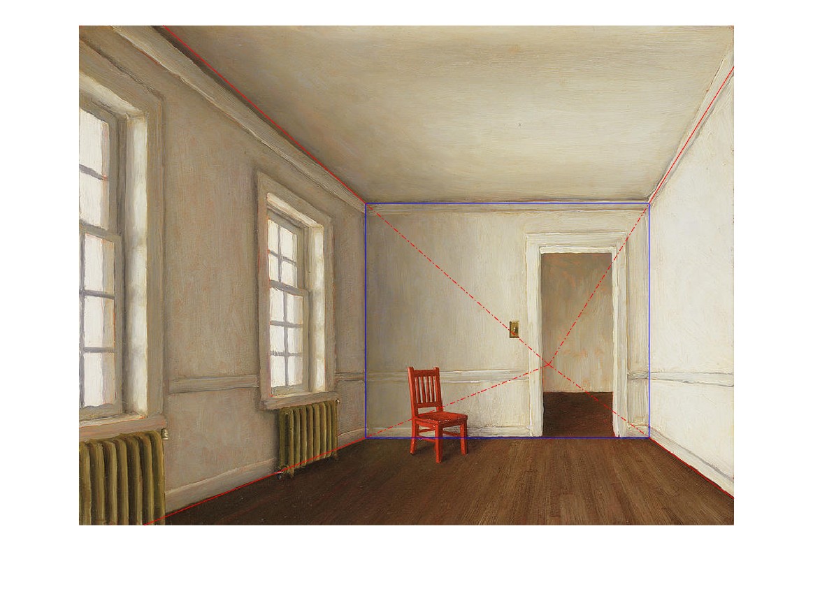
White Room - Harry Steen
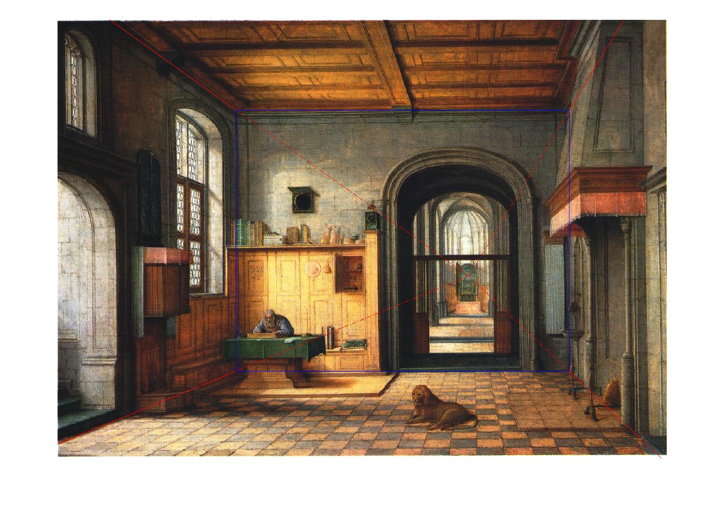
St. Jerome - Henry Steinwick
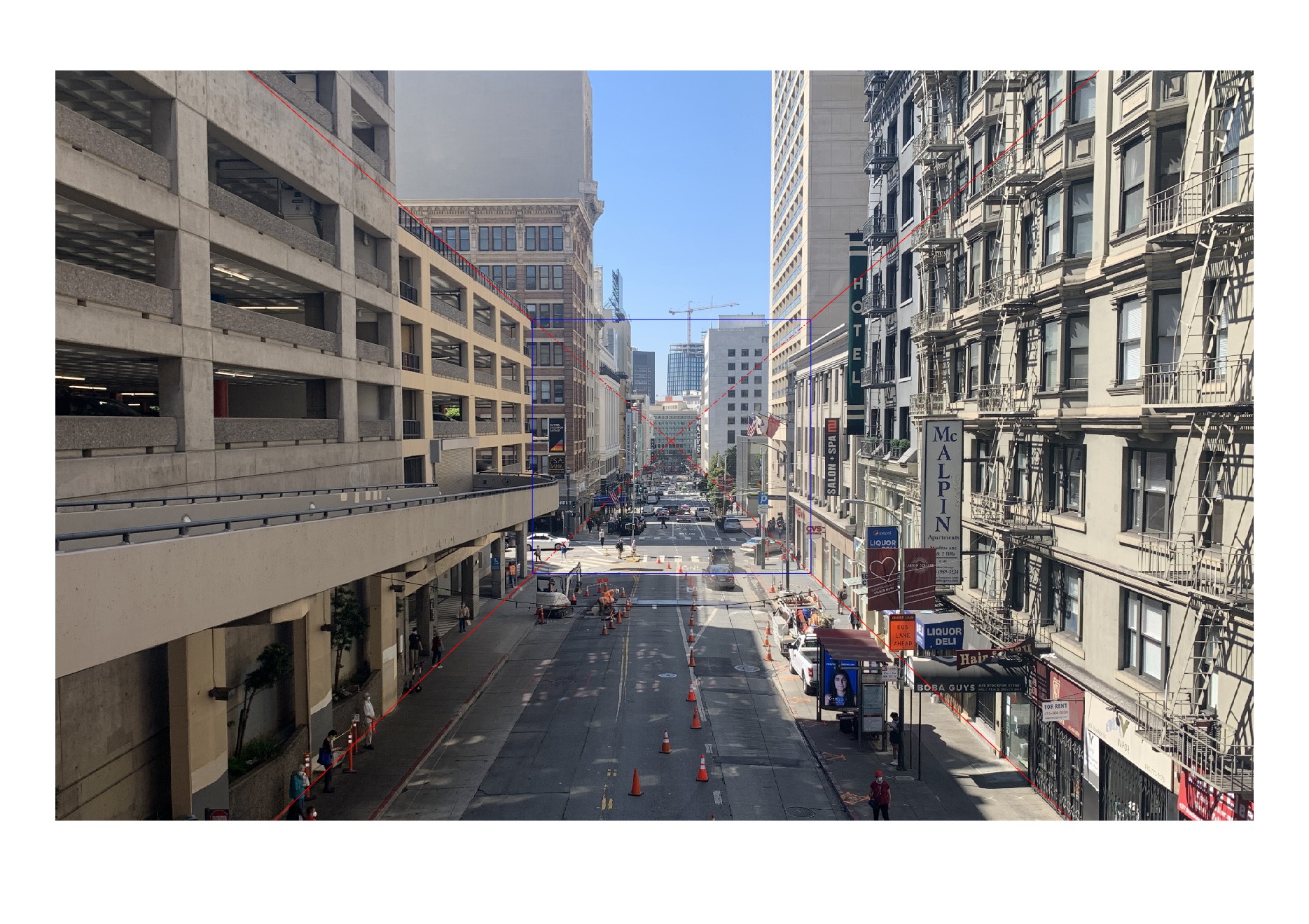
San Francisco
Now, we can reuse our code from project 4 to rectify each of the planes into rectangles. Note that this is necessary because all the planes other than the back wall appear as trapezoids in one point perspective. This process involves taking the 4 corners of each plane and computing the homography matrix that maps them to the corners of a rectangle. Once we have the matrix, we can map the full plane into a rectangle. The back wall dimensions are used for the height and width, and the depth is estimated (as we do not know the focal length of the cameras used for each image). Once we have our 5 rectangular planes, we can use MATLAB's built-in warp function to piece them together into a 3D model. Here are some "novel" viewpoints of each of the images:
Acapella Show
Original
View 1
View 2
White Room - Harry Steen
Original
View 1
View 2
St. Jerome - Henry Steinwick
Original
View 1
View 2
San Francisco
Original
View 1
View 2
These images do not quite capture the full beauty of this reconstruction; let's take a look at some video tours-into-the-pictures!
Acapella Show
White Room - Harry Steen
St. Jerome - Henry Steinwick
San Francisco
Bells and Whistles
You may have noticed that 3 of the 4 reconstructions contain protruding foreground objects. We will discuss those now. There are a few steps involved in creating additional planes for foreground objects-- object selection, inpainting, alpha masking, and calculating geometry.
Object Selection
I added a step that allows the user to select rectangles around their desired foreground objects, after selecting the back wall and vanishing point. Here are the foreground objects selected for each image (the acapella show does not have any obvious foreground objects, so it was excluded here):
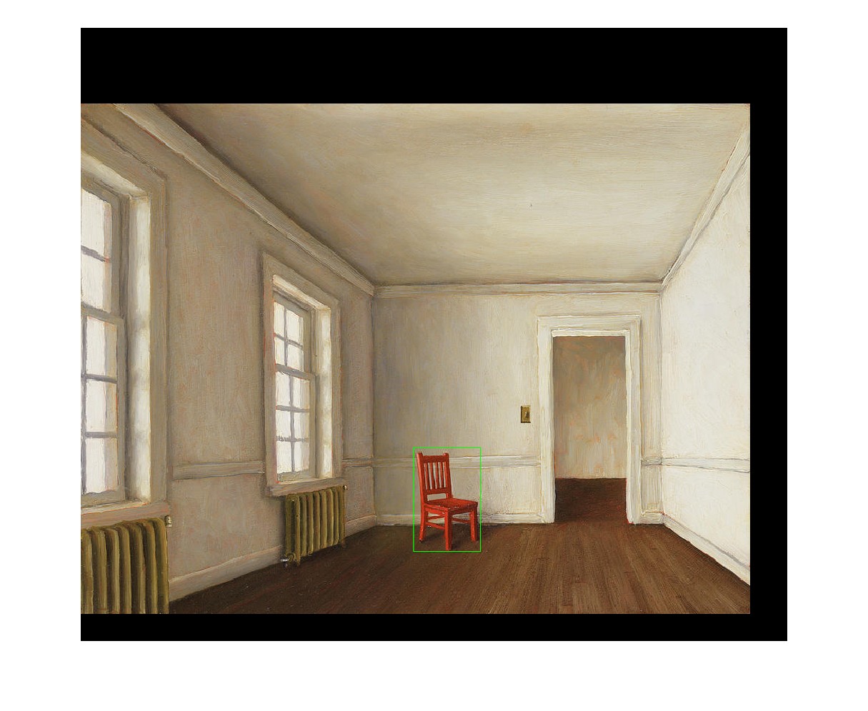
White Room - Harry Steen
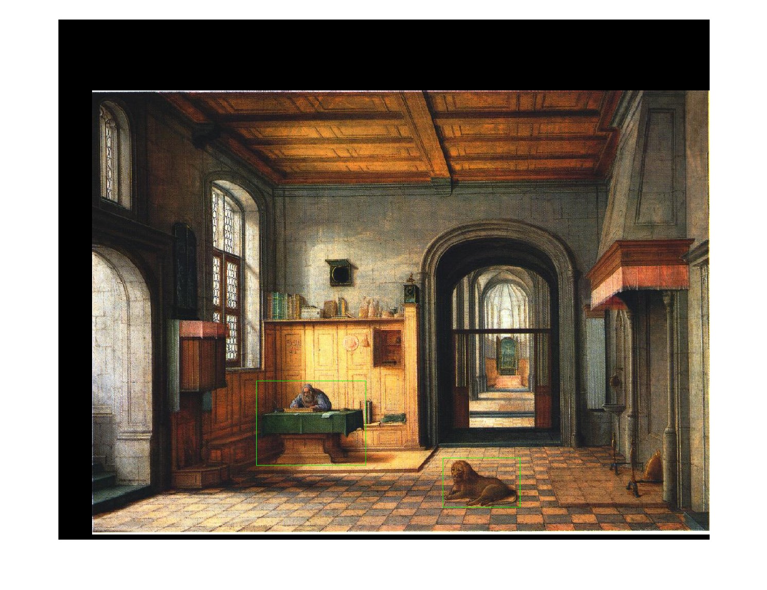
St. Jerome - Henry Steinwick
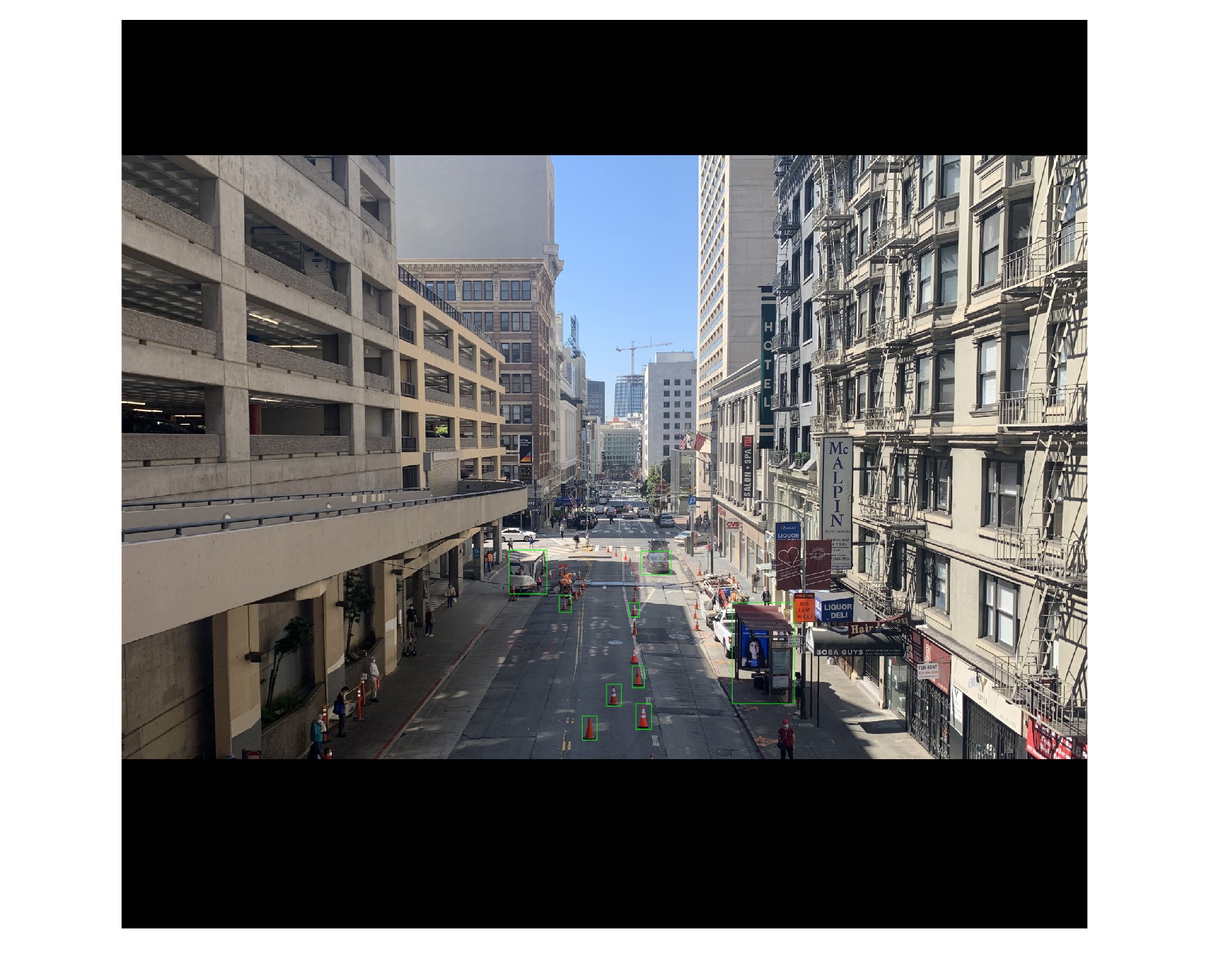
San Francisco
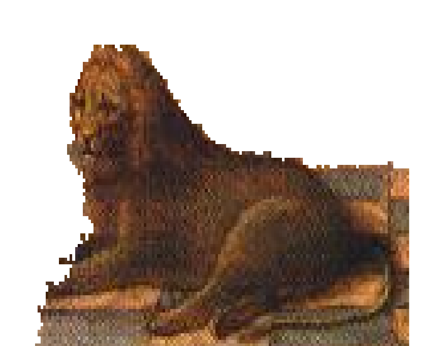
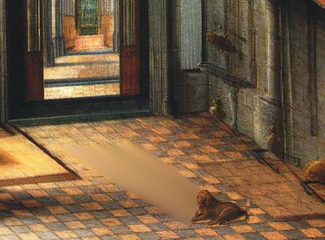
Inpainting
After selecting the foreground objects, we want to "inpaint" the space they take up in the original image so that they do not appear twice. The inpainting is done using MATLAB's region fill function, which interpolates pixel values in the desired regions using the surrounding pixels. Here is an example of inpainted foreground objects:
St. Jerome - Henry Steinwick
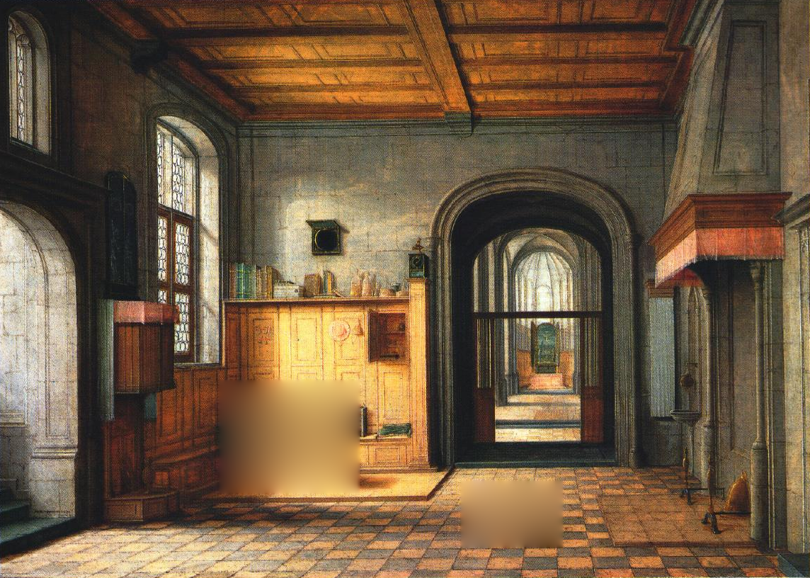
Foreground Objects Inpainted
Alpha masking
Another thing we want to take into account is the shapes of the objects themselves. Most objects are not perfect rectangles, so we need some way to "cutout" the natural shape of our foreground objects. We use MATLAB's grabcut function to auto-detect the object and create an alpha mask for it, setting the background transparent. Here is an example of this in action:
No grabcut
Grabcut
Calculating Geometry
Finally, we use the homography computed earlier to determine the object's location, and use similar triangle geometry to determine the object's height. Now we have all the information we need to create a new plane parallel to the back wall and place our object on it.
Foreground Object Example
Please scroll back up to the views and gifs of the picture tours to observe the inclusion of foreground objects. The effect is particularly noticeable in the traffic cones in the San Francisco image-- some cones were chosen as foreground objects and others were not. The cones that were selected look much better than the ones that were not, as they are no longer treated as part of the ground plane. Another thing to note is that the deeper cones appear to have the same height as the shallower cones, even though the shallower cones look bigger in the image. This is exactly what we hope to see, and perspective geometry prevails yet again.
Summary
This project was really fun, but unexpectedly tricky. I faced a lot of issues trying to get the 3D constructions set up correctly, with the orientations of the different planes and correct placements in the 3D space. The foreground objects were a whole other can of worms, as it was quite tricky to calculate the correct placements and heights and map it all into 3D. All in all, I think all the effort was worth it, as the final result might be one of my favorites from this whole semester.
Project 2: Light Field Camera
Now we will shift gears into depth refocusing and aperture adjustment using light field data. The datasets used here are very large and will thus not be included here-- only the results. If you desire to see the original datasets in their entirety, please visit this website:
Stanford Light Field ArchiveFor this project, I am using the datasets labelled "Chess" and "Tarot Cards and Crystal Ball (small angular extent)". These datasets consist of 17x17 grids of images. Each image is of the same scene, but with a slight shift in either the x or y direction.
Part 1: Depth Refocusing
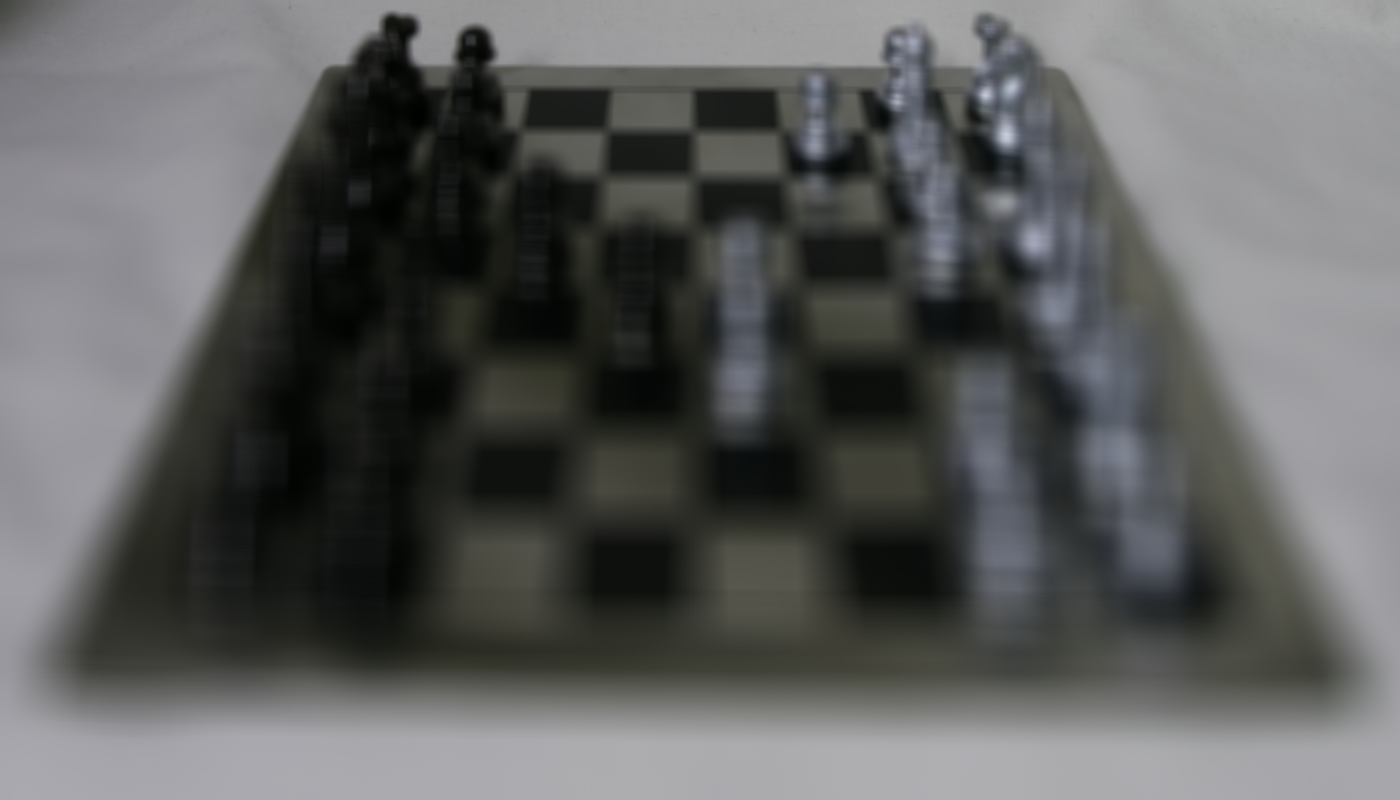
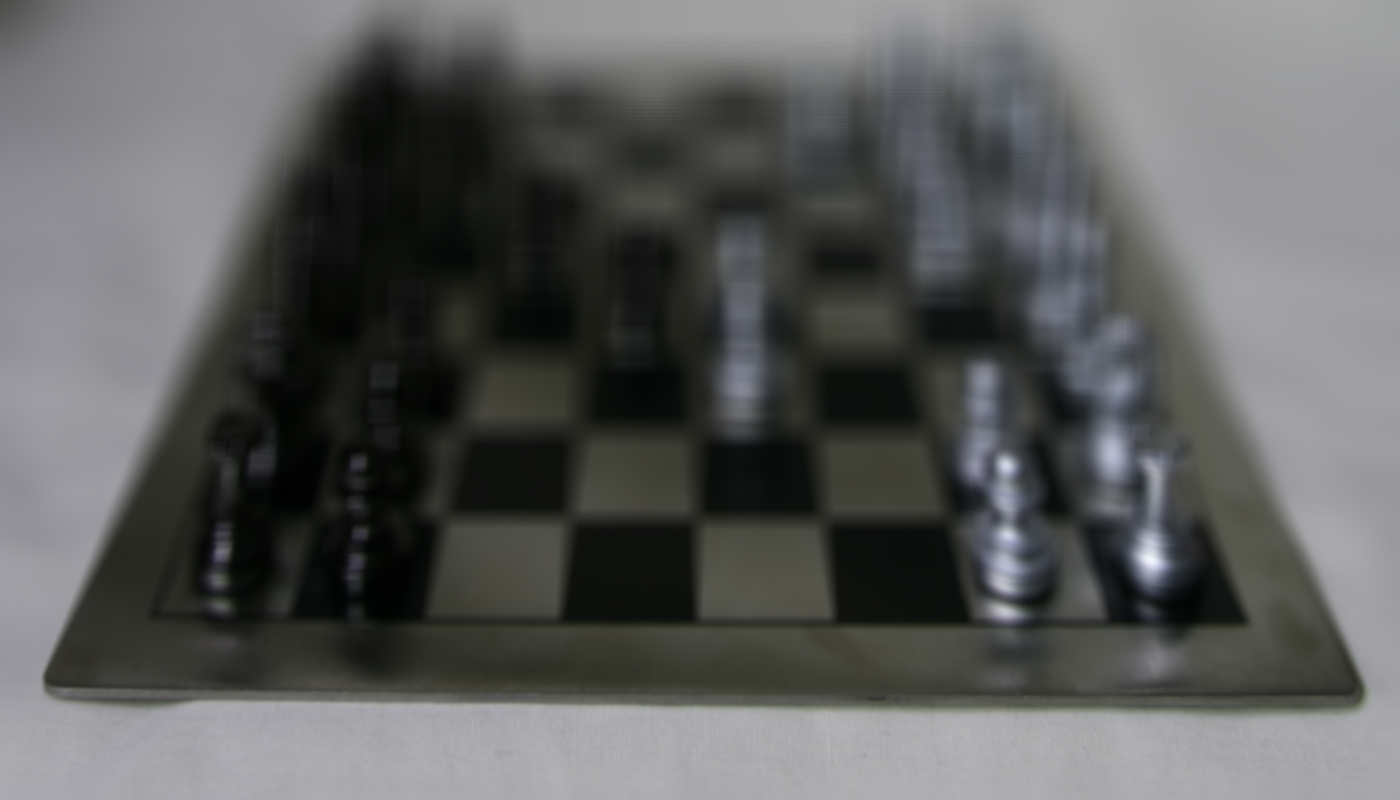
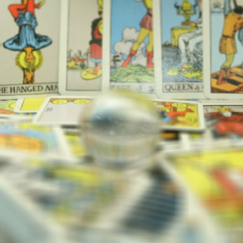
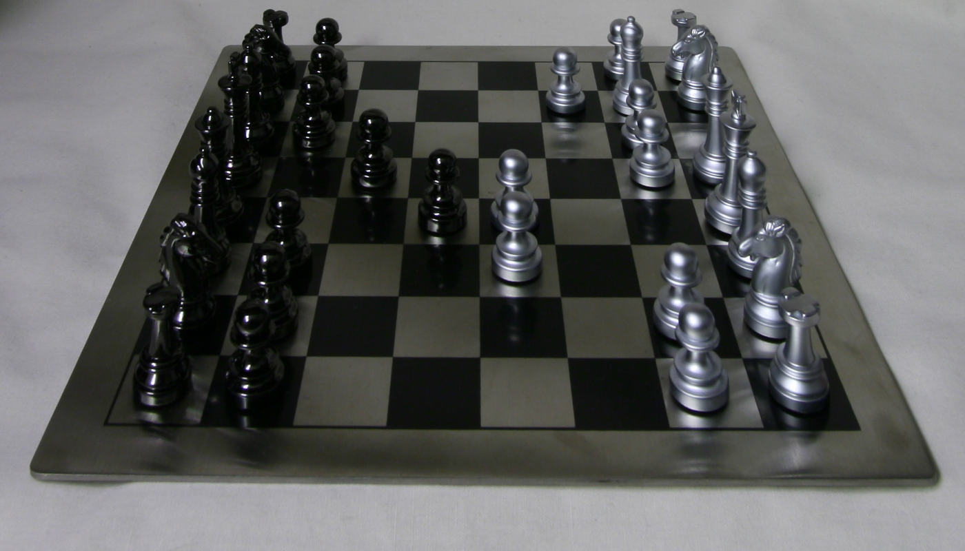
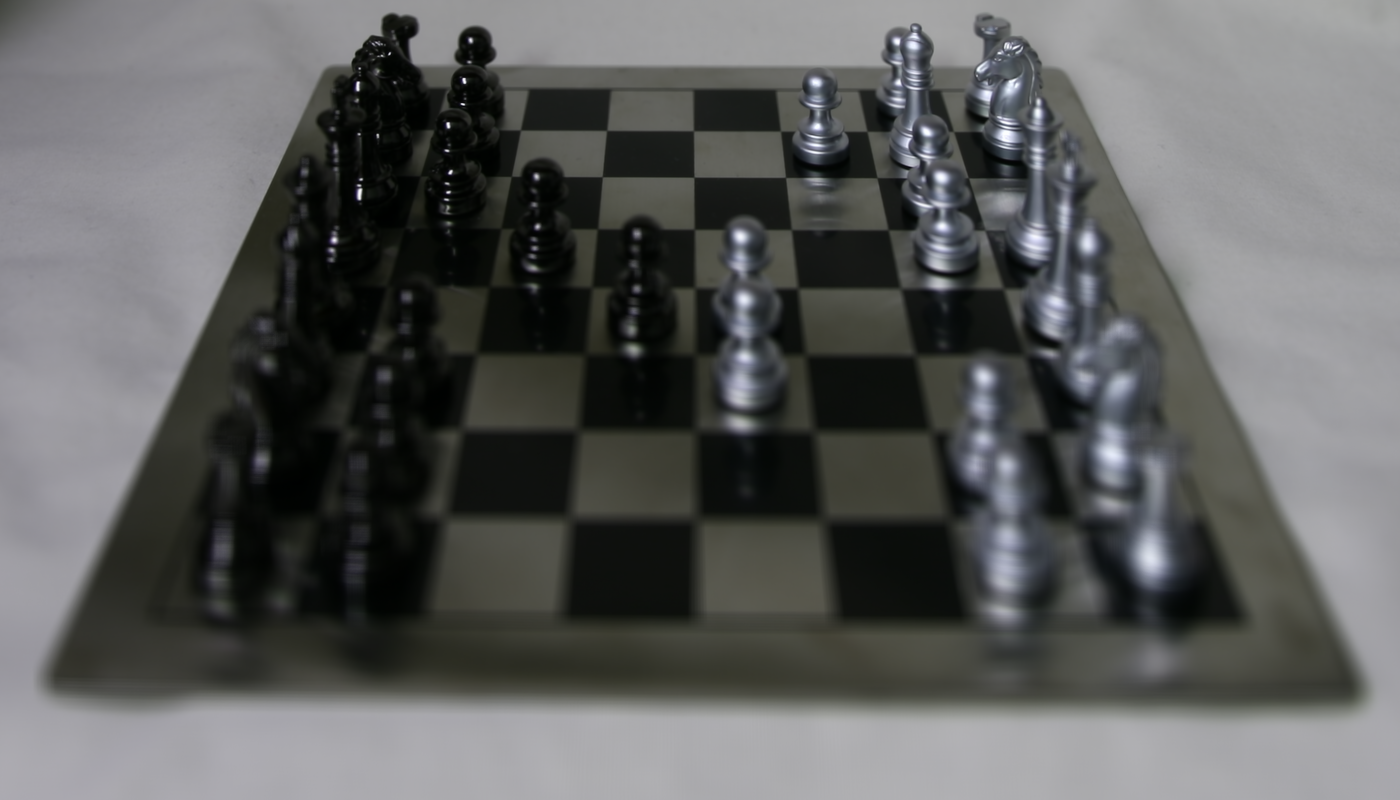
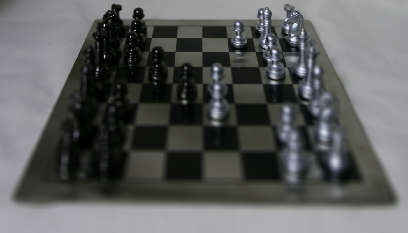
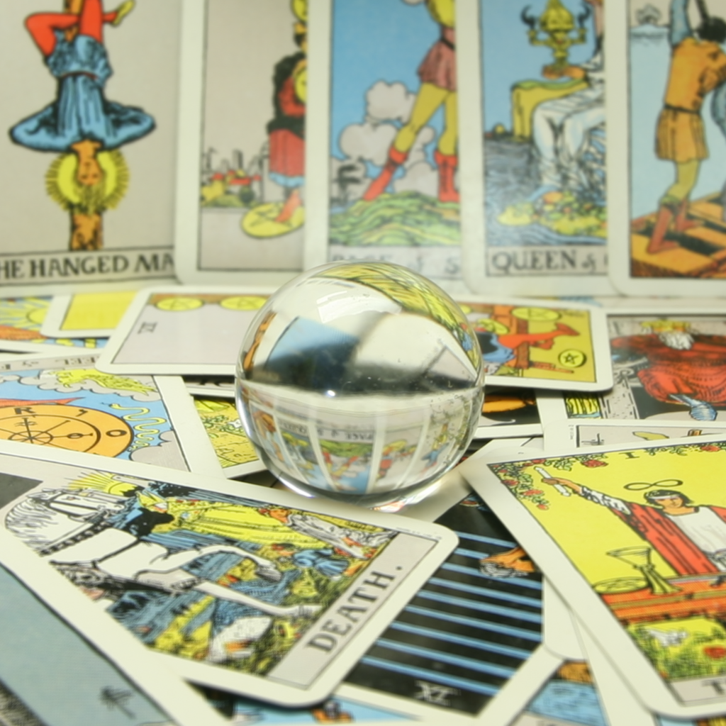
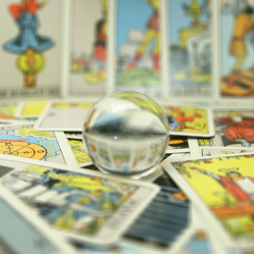
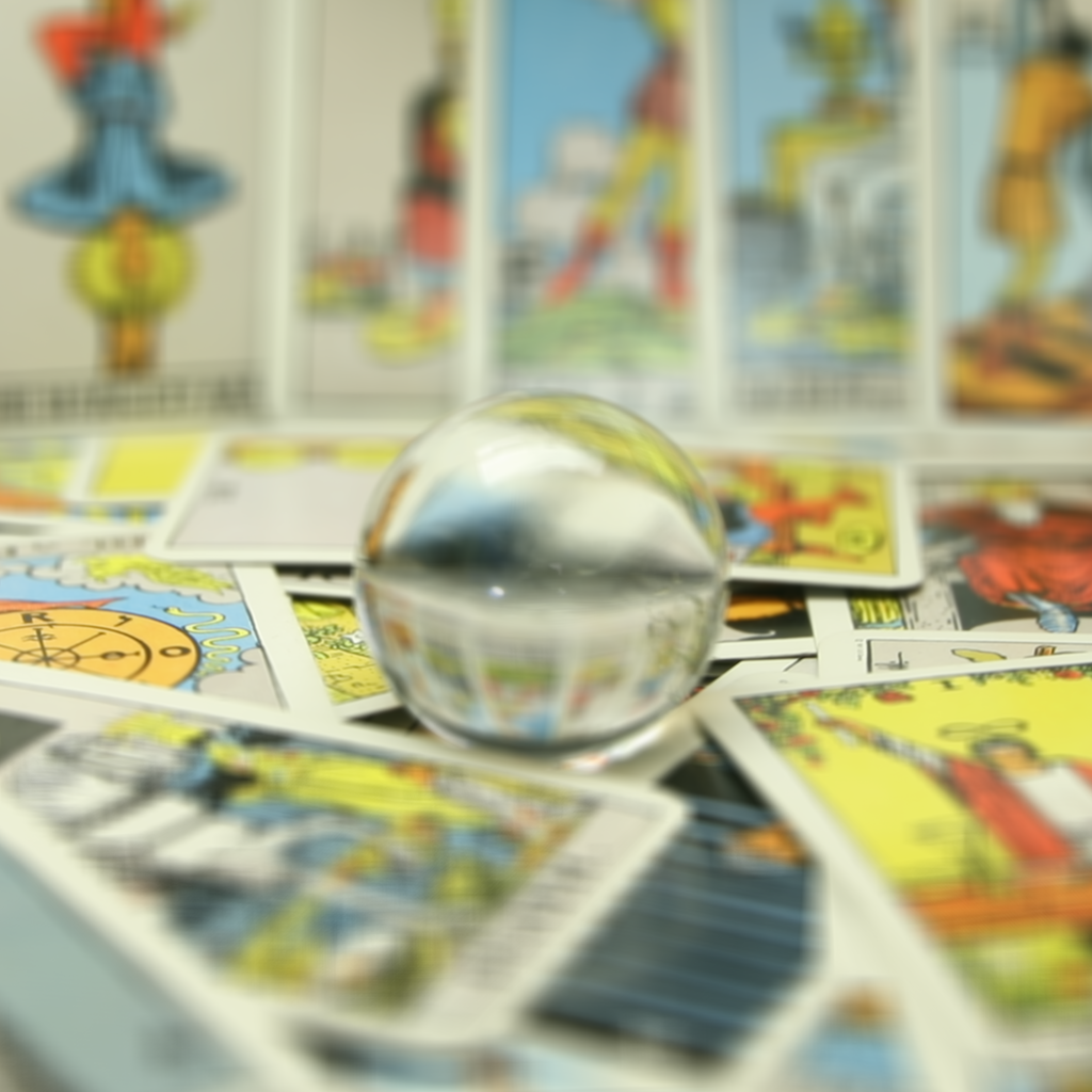
We can use our grids of images to simulate depth refocusing. If we were to simply average over all the images, we would get an image that focuses on a certain region of the image, typically the deepest parts. This is because the slight shifts in the x and y directions cause a significant shift in the foreground objects, but not nearly as much of a shift on the deeper objects. Here is a basic averaging over all the images in the chess dataset and the crystal ball dataset:
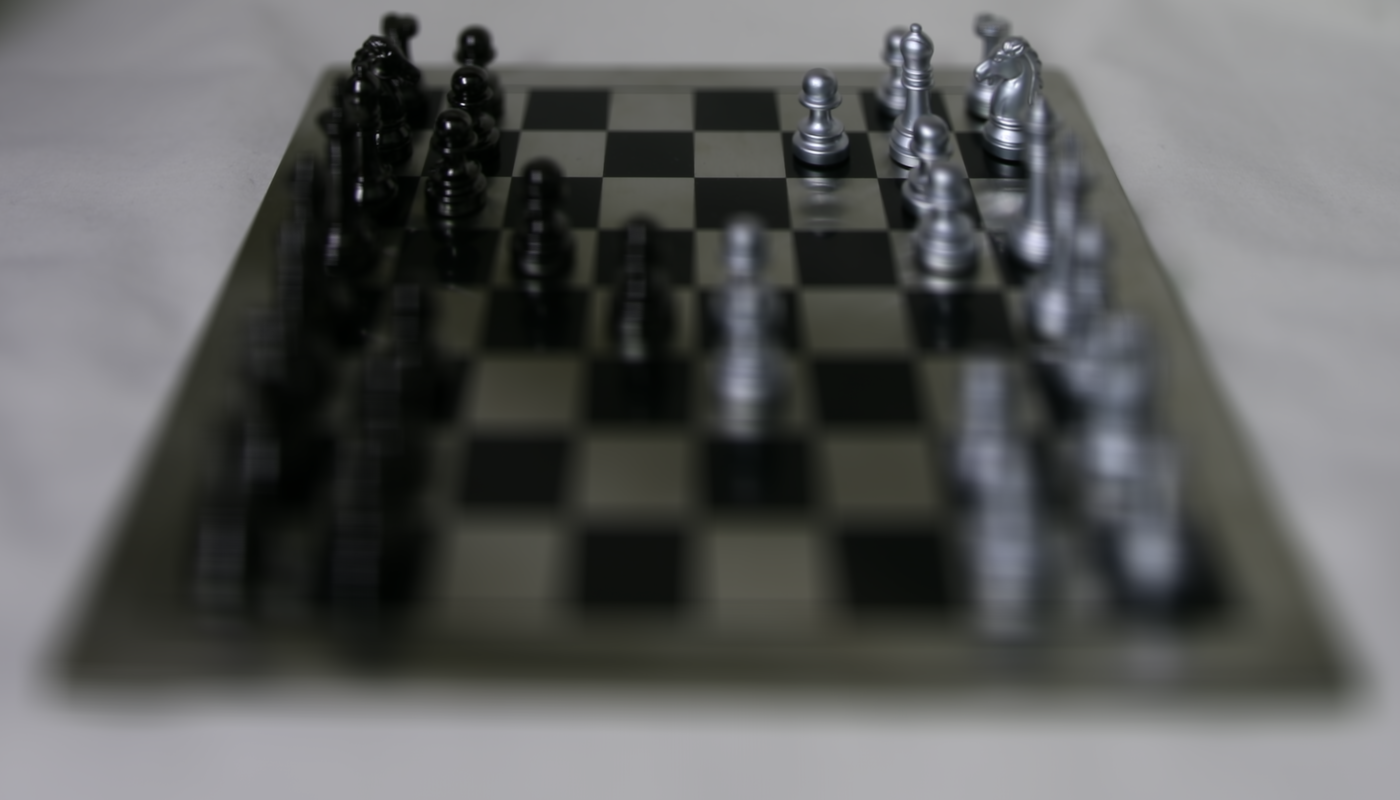
Chess
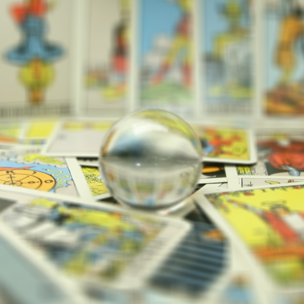
Crystal Ball
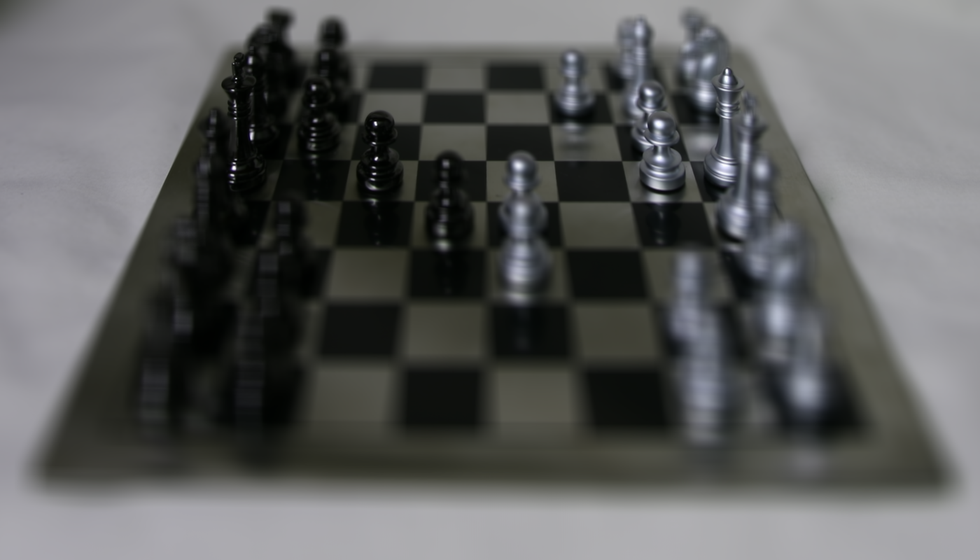
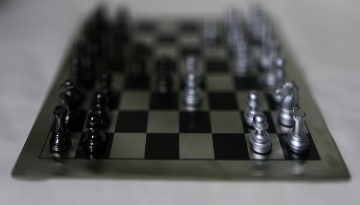
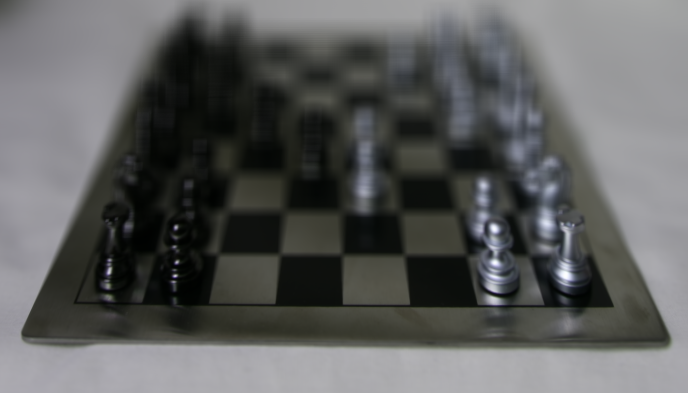
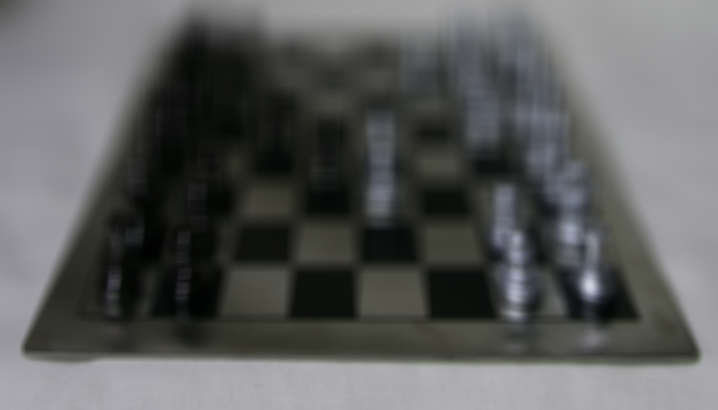
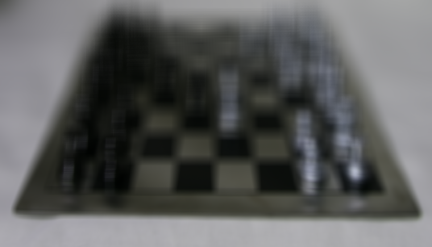
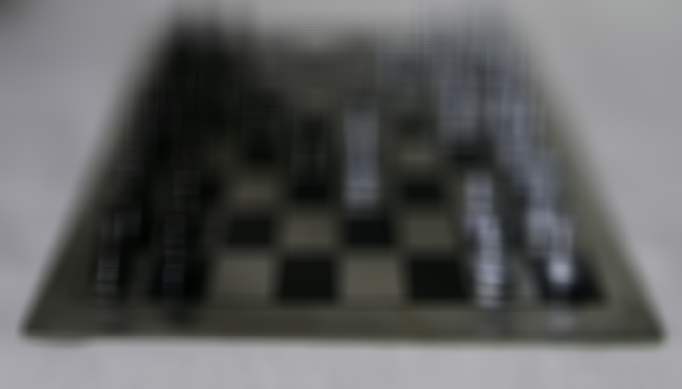
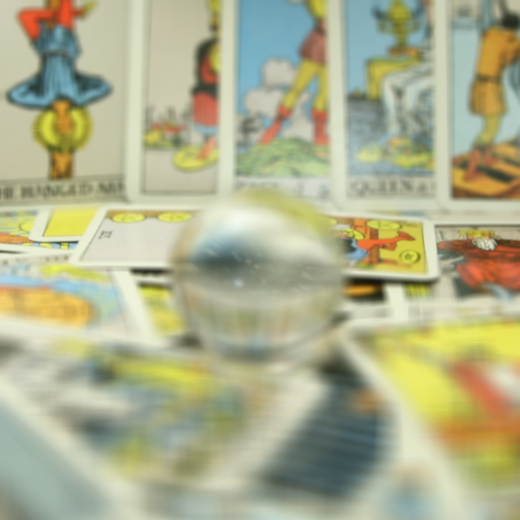
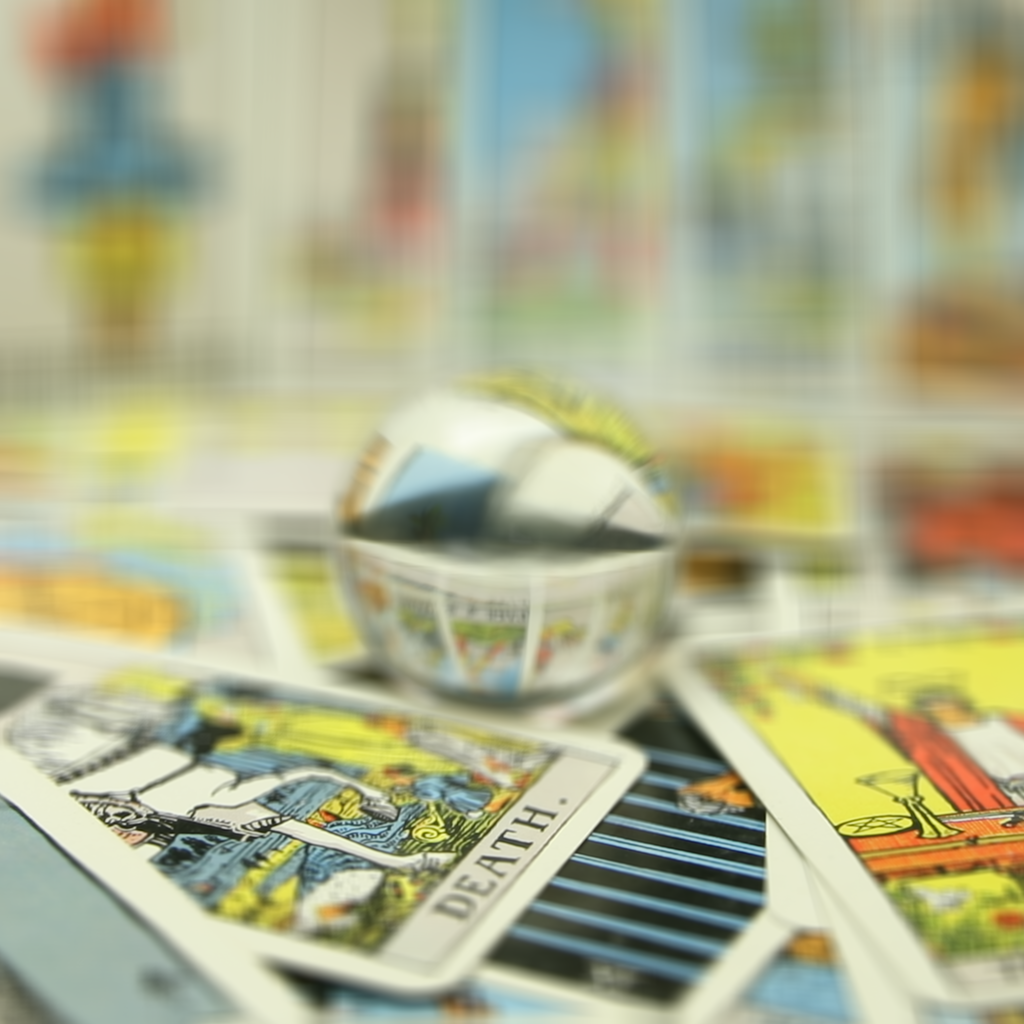
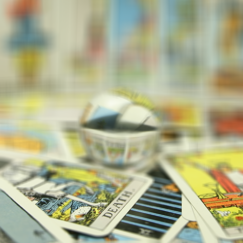
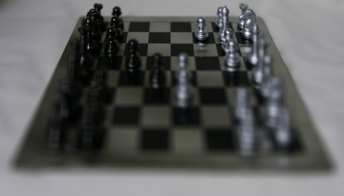
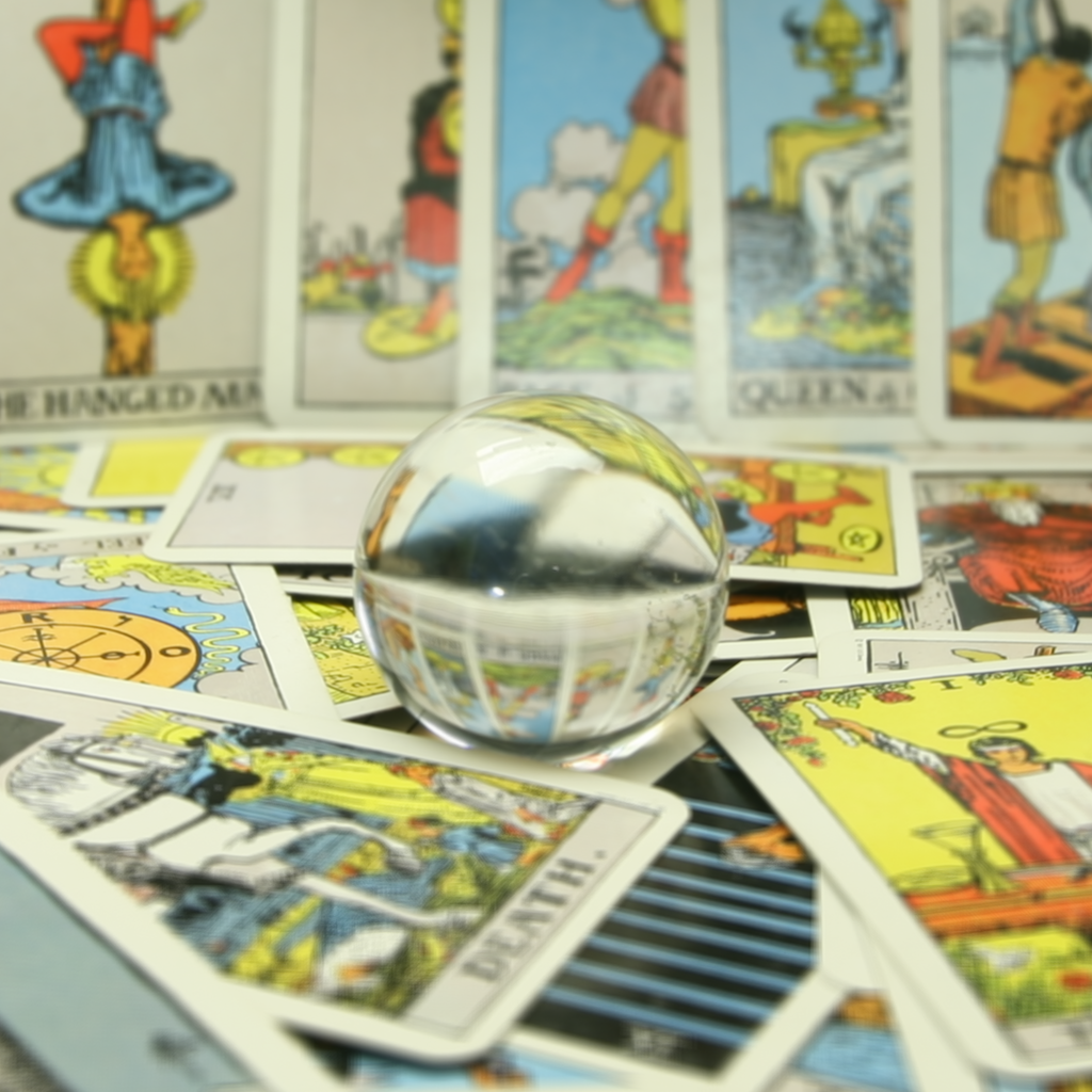
We can shift the focus in these images by shifting the images before averaging them. To do this, we compute the (x,y) coordinate shifts of each image, relative to the center image. Then, we can apply varying proportions (c) of this shift to the images and average them. I used proportions from the range [-0.5, 1.0] for both datasets. This has the effect of refocusing on different depths of the images:
Chess:
c=-0.5
c=-0.4
c=-0.3
c=-0.2

c=-0.1
c=0.0
c=0.1

c=0.2

c=0.3

c=0.4
c=0.5
c=0.6
c=0.7
c=0.8
c=0.9
c=1.0
Crystal Ball:

c=-0.5
c=-0.4
c=-0.3

c=-0.2

c=-0.1
c=0.0

c=0.1

c=0.2

c=0.3

c=0.4
c=0.5
c=0.6

c=0.7

c=0.8

c=0.9

c=1.0
Here are some gifs that showcase the refocusing a bit better:
Chess
Crystal Ball
Part 2: Aperture Adjustment
We can also use this dataset to very easily create images that mimic different apertures. To do this, we need to average over different "radii" of the dataset. The smallest aperture corresponds to just the center image by itself. The next smallest aperture corresponds to the average of all images that form a 3x3 grid around the center. We continue this until we reach the largest aperture, which is simply the average of the entire 17x17 grid. Here is what that looks like:
Chess:
1 image

9 images

25 images
49 images
81 images

121 images

169 images
225 images

289 images
Crystal Ball:

1 image
9 images
25 images

49 images

81 images
121 images
169 images

225 images

289 images
Again, we have some gifs to show off this effect a bit more:
Chess

Crystal Ball
Part 3: Summary
This project showed me that light fields capture a lot of information that is not quite present in conventional camera captures. The directional information encoded into light fields allows for useful and fascinating image manipulations even after the images have been captured, such as the depth-refocusing and aperture adjustment we saw here. These are subtle yet beautiful effects that I feel could be easily overlooked, but they add a lot potential variety into image captures.